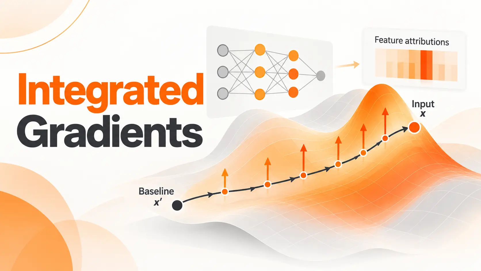
Integrated Gradients: How It Works and Examples

Integrated Gradients is a feature attribution method that explains how individual inputs contribute to a neural network's prediction. It compares the original input with a chosen baseline and calculates gradients along the path between them. The result shows which pixels, words, or numerical features support or oppose a selected model output.

In Explainable AI, I find Integrated Gradients especially useful when a neural network makes a prediction but gives little indication of which input information influenced it. A good attribution map can reveal whether an image classifier focuses on the object itself or on surrounding details. The important part is understanding what those highlighted regions mean and how the chosen baseline affects the explanation.

Integrated Gradients Example

Consider an image classification model that identifies a dog in a photograph.

The image contains a dog standing on grass, with trees and buildings in the background. The model predicts that the image belongs to the dog category.

That prediction tells us the result, but it does not reveal which visual features contributed to the model's output.

Integrated Gradients can produce an attribution map showing the contribution of individual pixels to the selected dog class score.

I would examine three visual elements together: the original photograph, the baseline image, and the resulting attribution map.

Original image: Shows the dog and its surroundings exactly as the model received them.

Baseline image: Provides the reference input against which feature contributions are measured. For this example, we can use a completely black image with the same dimensions.

Attribution map: Shows the calculated contributions of individual pixels to the difference between the selected model output for the original image and the baseline.

Suppose the strongest positive attributions appear around the dog's ears, face, and body. That would indicate those regions contribute positively to the selected dog class score relative to the baseline.

If substantial contributions appear in the background, I would investigate whether the model is also relying on environmental details.

This matters because the model could associate particular backgrounds with certain animals instead of learning visual patterns that generalize across different environments.

The attribution map does not prove that the model understands what a dog is. It provides evidence about how the selected output responds to the image relative to the chosen reference.

How Integrated Gradients Works

Integrated Gradients was introduced by Sundararajan, Taly, and Yan in their 2017 research paper, Axiomatic Attribution for Deep Networks.

The method addresses a limitation of ordinary gradient explanations: examining gradients only at the original input can miss important contributions when parts of a neural network have saturated.

Integrated Gradients instead considers gradients along a continuous path between a baseline and the actual input.

Selecting the Baseline and Input

The process begins with two inputs of the same structure.

The first is the original image that receives the model prediction. The second is a reference image called the baseline.

For our dog classification example, the baseline could be a black image.

The algorithm measures the change in the selected model output between these two inputs.

The baseline therefore defines the starting point of the explanation.

Creating Intermediate Inputs

Integrated Gradients constructs a sequence of intermediate images between the baseline and the original photograph.

At the beginning of the path, the image matches the baseline.

As the process advances, the intermediate images progressively approach the original input.

The standard method follows a straight path through the input feature space.

For an image with a black baseline, this can be visualized as a sequence that begins completely black and gradually reveals the original photograph.

The intermediate images are calculation points, not necessarily realistic photographs.

Calculating Gradients Along the Path

At multiple points along the path, the algorithm calculates how sensitive the selected model output is to small changes in each input feature.

For images, these features are pixel values.

Instead of evaluating only the gradient at the original image, Integrated Gradients accumulates gradient information across the path.

This captures contributions that a gradient calculated at a single point could miss.

Calculating the Final Attribution

The accumulated gradients are combined with the difference between the original input and the baseline.

Each feature receives an attribution value representing its contribution to the change in the selected model output.

A feature with a positive attribution supports that output difference. A feature with a negative attribution opposes it.

The resulting attribution values can then be visualized as a map or examined numerically.

Integrated Gradients explains the difference between the original input and the baseline, not the prediction in isolation.

That distinction is essential when interpreting the result.

Choosing an Integrated Gradients Baseline

Baseline selection is one of the most important decisions in Integrated Gradients.

The baseline represents the reference against which the original input is compared.

Changing that reference can change the attribution values even when the original image and trained model remain identical.

Black Image Baseline

A black image is a common starting point for image classification.

It sets the pixel values to zero in the input representation.

This choice makes the progression from baseline to original image easy to visualize.

However, a black image is not inherently a neutral reference for every model. Its meaning depends on preprocessing, pixel scaling, and the visual patterns learned during training.

A black image can also be far outside the model's training distribution.

I would use it as an initial comparison rather than assume it provides the most meaningful explanation.

Gray and Blurred Baselines

A gray image provides a different reference by assigning a constant intermediate intensity.

A blurred image preserves broad visual structure while removing finer details.

These choices answer different attribution questions.

Using a blurred baseline can help investigate how finer image details contribute to the selected output relative to a version that retains broader visual information.

However, neither approach guarantees that the baseline is representative of the absence of information.

The interpretation must always remain tied to the selected reference.

Comparing Multiple Baselines

For an important prediction, I would compare attribution maps generated using more than one defensible baseline.

If the same regions receive substantial contributions across different references, that provides useful evidence of consistency.

If the highlighted regions change dramatically, I would investigate why before relying on the explanation.

One subtle limitation is that a feature identical to its baseline value receives zero Integrated Gradients attribution by construction.

A zero attribution therefore does not automatically establish that the feature is irrelevant to the model.

This baseline dependence is an important reason to avoid treating a single attribution map as definitive.

Interpreting Integrated Gradients Attribution Maps

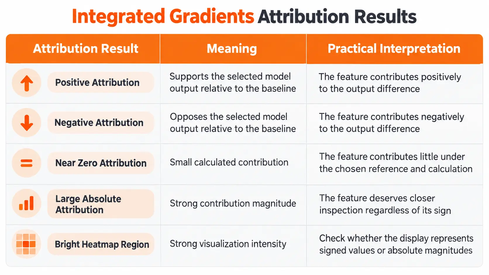
An Integrated Gradients attribution map displays how input features contribute to a selected model output relative to the baseline.

The underlying attribution values have signs and magnitudes.

Those numerical properties must be distinguished from the colors used to visualize them.

Positive and Negative Attributions

Return to the dog classification example.

A positive attribution around the dog's face indicates that those pixels contribute positively to the selected dog class output relative to the baseline.

A negative attribution indicates a contribution in the opposite direction.

These values are specific to the selected output.

If we change the target from the dog class to another animal class, the attribution map can change because the algorithm is now explaining a different model output.

I would always record the target class alongside the attribution map.

Attribution Magnitude and Heatmap Colors

A large attribution magnitude means the corresponding feature makes a larger contribution to the selected output difference under the chosen method.

However, visualization settings can change how that contribution appears.

Some heatmaps preserve the difference between positive and negative values through separate colors.

Others combine absolute attribution magnitudes, showing the strongest contributions without indicating whether they support or oppose the output.

For example, the TensorFlow Integrated Gradients tutorial demonstrates a visualization that sums absolute attribution values across image color channels.

This produces a useful importance mask, but the resulting intensity does not preserve the sign of each contribution.

I would inspect the color scale and aggregation method before interpreting a bright region as evidence supporting the predicted class.

Attribution Maps and Model Confidence

A highlighted region is not the same thing as a probability contribution unless the selected output and attribution calculation support that interpretation.

A model can expose class logits, probabilities, or another differentiable score.

Integrated Gradients attributes the specific output selected for analysis.

Therefore, changing from a class logit to a predicted probability changes the quantity being explained and can change the attribution values.

I prefer to identify the exact output before examining the map rather than treat every attribution as a contribution to confidence.

Integrated Gradients with TensorFlow and PyTorch

TensorFlow and PyTorch both support Integrated Gradients, although their implementation workflows differ.

The underlying method remains the same: choose a differentiable model output, define a baseline, calculate gradients along the path, and combine those gradients into feature attributions.

Integrated Gradients in TensorFlow

TensorFlow provides an official tutorial demonstrating Integrated Gradients for image classification.

The implementation uses automatic differentiation to calculate gradients at intermediate points between the baseline and the original image.

For a practical workflow, I would begin with a trained image classifier and verify that the image preprocessing matches what the model expects.

Next, I would select the target class and construct a baseline image.

The intermediate images are then evaluated by the model, and their gradients are accumulated to calculate the attribution values.

Finally, the results can be visualized as an attribution map overlaid on the original photograph.

I would keep the signed attribution values available even when displaying a simplified heatmap. That prevents information from being lost during visualization.

Integrated Gradients in PyTorch

PyTorch users can implement Integrated Gradients through Captum, a model interpretability library built for PyTorch.

Captum provides an IntegratedGradients class that accepts a model's forward function and calculates attributions for selected inputs.

The implementation supports configuring baselines, target outputs, integration steps, and numerical approximation methods.

It can also return a convergence delta to help evaluate the numerical calculation.

For an image classification project, I would first verify the model's expected input representation and target class.

Then I would generate attributions, inspect the convergence result, and visualize the contributions.

Using Captum avoids rebuilding the integration procedure from the beginning while preserving control over the important settings.

Choosing the Number of Integration Steps

Integrated Gradients requires a numerical approximation of the continuous gradient integral.

The number of integration steps controls how many points are evaluated along the path.

Using more steps can improve numerical accuracy, but it increases computation time and memory requirements.

I would begin with a manageable number of steps and inspect the convergence delta.

If the approximation error remains substantial, I would increase the steps and evaluate the result again.

A larger number of steps is not automatically necessary for every model. The appropriate setting depends on the prediction function and the numerical method.

Completeness and Convergence Delta

One of the defining properties of Integrated Gradients is Completeness.

It states that the sum of feature attributions equals the difference between the selected model output for the original input and the baseline.

This provides a useful numerical consistency check.

Consider a hypothetical model that assigns a selected output score of 0.80 to an image and 0.20 to its baseline.

The difference is 0.60.

Under the Completeness property, the individual Integrated Gradients attributions should sum to 0.60 when the integral is calculated exactly.

In practice, numerical integration produces an approximation.

Understanding Convergence Delta

Convergence delta measures the discrepancy between the sum of calculated attributions and the corresponding model output difference.

A small absolute convergence delta indicates that the numerical approximation closely satisfies Completeness.

A larger discrepancy suggests the integration calculation needs further examination.

Captum can return this value as part of its Integrated Gradients output.

I would use it to assess whether the numerical calculation is sufficiently accurate for the application.

However, a small convergence delta does not prove that the explanation is meaningful or trustworthy.

The attribution can satisfy the mathematical property while still depending on a questionable baseline or highlighting patterns unrelated to the intended task.

Numerical accuracy and explanatory reliability are separate considerations.

Integrated Gradients for Images, Text, and Tabular Data

Integrated Gradients applies to differentiable models beyond image classification.

Its interpretation depends on the input representation and the model output being explained.

Image Classification

For image models, the method assigns contributions to pixel values.

These can be visualized as heatmaps showing how different image regions relate to a selected classification score.

I would use this view to investigate whether the model relies on the intended object or on surrounding visual patterns.

The attribution map does not automatically provide object boundaries or prove that the model recognizes meaningful visual concepts.

Text Classification

In natural language processing, Integrated Gradients can help investigate which words or tokens contribute to a selected prediction.

Consider a sentiment classifier that labels a product review as negative.

An attribution analysis can help identify which token representations contribute to the negative sentiment score relative to the chosen reference.

There is an important technical distinction: token identifiers are discrete values and cannot be meaningfully interpolated as continuous inputs.

For transformer models, the method can instead attribute predictions through differentiable embedding representations.

Captum provides LayerIntegratedGradients for this type of analysis.

Individual embedding contributions can then be aggregated into token level scores for interpretation.

Tabular Data

For structured datasets, Integrated Gradients assigns contributions to numerical input features or suitable differentiable representations.

A neural network predicting customer churn could be examined using features such as account activity, subscription duration, and usage frequency.

The explanation would show how those input values contribute to the selected output relative to the baseline.

I would pay particular attention to feature scaling and reference selection because numerical features can have very different ranges and meanings.

Categorical features represented through embeddings also require careful interpretation of the resulting attributions.

Integrated Gradients vs Saliency Maps and SHAP

Integrated Gradients belongs to the broader family of feature attribution methods, but its calculation differs from standard gradient saliency and SHAP.

Integrated Gradients vs Saliency Maps

A basic gradient saliency map examines the sensitivity of a model output to changes in the input at the original observation.

Integrated Gradients accumulates gradients along the path from a baseline to the observation.

This matters when the model's gradient at the original input is small even though the feature contributed to the difference in model output along the path.

By integrating gradients, the method can capture contributions that a single local gradient does not reveal.

However, both approaches depend on the differentiability of the selected model output.

Integrated Gradients vs SHAP

SHAP uses a feature attribution framework based on Shapley values.

Its explanations depend on the selected reference or background formulation and the assumptions used to represent feature contributions.

Integrated Gradients instead calculates gradient contributions along a path from a baseline to the original input.

I would consider Integrated Gradients when working with a differentiable neural network and needing an explanation relative to a defined reference.

SHAP is worth evaluating when its attribution framework better matches the explanation objective or when the model architecture benefits from a specialized SHAP implementation.

The methods do not provide interchangeable explanations.

Differences between their results can reflect distinct assumptions, references, and attribution calculations rather than an error in either technique.

Limitations of Integrated Gradients

Integrated Gradients has useful mathematical properties, but those properties do not eliminate practical interpretation challenges.

Baseline Sensitivity

The explanation depends on the selected reference input.

Different baselines can produce different attribution maps for the same prediction.

I would compare defensible baseline choices before presenting an explanation as evidence of model behavior.

Unrealistic Intermediate Inputs

The standard method moves along a straight path between the baseline and the original input.

Intermediate points on that path can fall outside the distribution of examples the model encountered during training.

The algorithm still evaluates gradients at those points.

As a result, attributions can reflect model behavior on unrealistic intermediate inputs.

A visually plausible endpoint does not guarantee that the entire integration path is realistic.

Attribution Without Causality

Integrated Gradients identifies feature contributions to a model output difference.

It does not establish that changing those features in the real world would cause a particular outcome.

For example, a medical image attribution map can show which pixels contribute to a diagnostic model's score. It cannot establish that the highlighted region represents a verified clinical cause.

That requires separate domain evidence and validation.

Limited Information About Feature Interactions

Standard Integrated Gradients assigns contributions to individual input features.

It does not directly provide a complete explanation of how feature combinations interact.

A network can depend on relationships between pixels or groups of variables that are difficult to understand from individual attribution values alone.

I would use additional inspection methods when interactions are central to the question.

Evaluating Integrated Gradients Explanations

A convincing attribution map is not enough to establish that the explanation is reliable.

I would evaluate whether the results remain meaningful under controlled changes to the explanation setup.

First, I would compare different baseline choices and examine whether the primary attributed regions change substantially.

Next, I would inspect the convergence delta and test whether increasing the number of integration steps materially changes the calculated values.

I would also compare explanations for several inputs representing the same class, rather than forming conclusions from one selected image.

For image classification, another useful test is to examine whether the attributions change when the model parameters are altered. An explanation that remains largely unchanged after substantial model changes deserves further investigation.

Finally, I would compare highlighted regions against the actual task and available domain knowledge.

If an animal classifier repeatedly highlights the background instead of the animal, that finding can guide further investigation into the training dataset and learned patterns.

The goal is not to force the explanation to match human expectations. It is to determine whether it accurately characterizes the model's behavior and exposes patterns worth examining.

Conclusion

Integrated Gradients provides a structured method for understanding how input features contribute to neural network predictions.

By integrating gradients between a baseline and the original input, it produces attribution values that can be interpreted through numerical scores or visual maps.

I consider three factors essential for using the method effectively: selecting a defensible baseline, interpreting the signed attributions correctly, and checking the numerical approximation through Completeness and convergence delta.

A useful explanation should also remain connected to the model's actual behavior rather than simply produce an attractive heatmap.

Integrated Gradients becomes most valuable when it helps identify what a model relies on, where its behavior deserves further investigation, and which conclusions the attribution method cannot establish.

FAQ

Can I use Integrated Gradients without a GPU?

Yes. Integrated Gradients can run on a CPU when the model and required operations are supported. Execution time depends on model complexity, input dimensions, and integration steps. Large neural networks can require substantial computation, making GPU acceleration useful for repeated explanations.

Can I explain a model that I can only access through an API?

Standard Integrated Gradients requires gradients of the selected output with respect to the input. An API that returns predictions without providing gradient access is insufficient for direct implementation. In that situation, a method designed for prediction only access is more appropriate.

Can I use Integrated Gradients with a transformer model?

Yes. Integrated Gradients can explain differentiable transformer models. For token based inputs, attribution is performed on suitable continuous representations such as embeddings rather than directly on discrete token identifiers. The selected target and reference representation must be defined consistently.

Why do some important pixels have zero attribution?

A pixel can receive zero attribution when its value matches the corresponding baseline value, even when that pixel participates in the model's prediction function. Zero can also result from the gradient behavior along the chosen path. The result should be interpreted relative to the baseline and target output rather than as proof of complete irrelevance.

Can I save Integrated Gradients results for later comparison?

Yes. Attribution values and visualizations can be stored alongside the model version, input, baseline, target output, preprocessing configuration, and integration settings. Preserving these details supports reproducible comparisons. Results from different configurations should not be treated as directly equivalent without accounting for those differences.