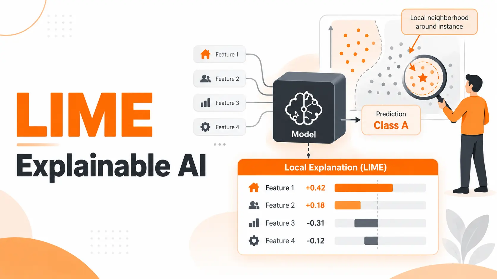
LIME Explainable AI: How It Works, Examples, and Python

LIME Explainable AI helps explain why a machine learning model made a particular prediction. Short for Local Interpretable Model Agnostic Explanations, LIME examines how a model responds to changes in an individual input and builds a simpler explanation of its behavior. It can explain predictions from complex models without requiring access to their internal architecture.

Within Explainable AI, LIME is particularly useful when a prediction deserves closer inspection. I find the most valuable question is not simply which features the model considers important, but which features influenced the specific result being investigated. Understanding that difference is essential for interpreting LIME correctly.

How LIME Explains Machine Learning Predictions

Imagine a bank uses a machine learning model to identify suspicious transactions. The model flags a payment, but the prediction alone does not explain which details influenced its decision.

LIME investigates that individual transaction by creating modified versions of its input features. It submits those variations to the original model and observes how the predicted probability changes.

The process follows four stages.

1. Selecting a prediction

LIME begins with one observation and the model prediction that needs explanation. In our example, this is a transaction flagged as potentially fraudulent.

2. Generating modified samples

LIME creates variations of the original input. These samples allow it to observe how the model responds when feature values change.

3. Weighting nearby observations

The generated samples receive weights based on their similarity to the original observation. Samples considered closer have greater influence on the explanation.

4. Fitting a local surrogate model

LIME fits an interpretable model, typically a sparse linear model, to approximate the original model's predictions in that neighborhood. Its coefficients provide the feature contributions presented in the explanation.

The original prediction model remains unchanged throughout this process. LIME studies its responses rather than retraining it.

The result is a local explanation. It describes how the model behaves around the selected observation, not how every prediction across the dataset is produced.

LIME Explanation Example

Consider a fraud detection model that assigns an 82% probability to the suspicious transaction class for a particular payment.

The transaction involves an unusually large purchase made from a new device. However, the recipient has appeared in earlier transactions, and the account was accessed from a familiar location.

LIME can help identify which conditions support the fraud prediction and which conditions work against it.

The following example uses illustrative feature weights to demonstrate how a LIME explanation is interpreted. These are not measured results from an executed model.

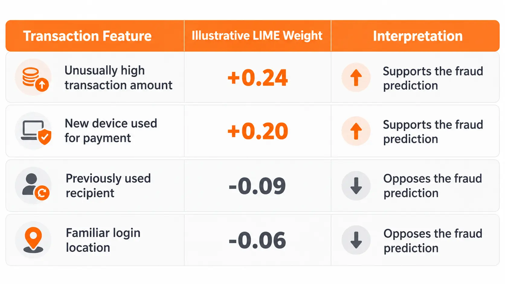
The two positive contributions suggest that the model's fraud prediction is locally supported by the transaction amount and unfamiliar device.

The negative contributions indicate that the familiar recipient and login location pull the local explanation in the opposite direction.

These weights are not direct changes in fraud probability. They are contributions within LIME's local surrogate model and depend on how the features are represented.

The model's 82% prediction and LIME's explanation are separate outputs. One reports the original model's estimated probability, while the other approximates how selected features relate to that prediction.

This distinction prevents a misleading interpretation of the results.

LIME also does not establish whether the transaction is actually fraudulent. It explains the prediction made by the model, not the underlying truth of the event.

LIME Python Tutorial

Python provides an accessible way to apply LIME to trained machine learning models. The original LIME library supports tabular data, text classification, and image classification.

For this walkthrough, I would use a transaction classification dataset and a Random Forest classifier. The aim is to explain one prediction while preserving the preprocessing and feature structure used during training.

Preparing the Machine Learning Model

Start with a labeled transaction dataset containing features such as transaction amount, account age, device status, and recent transaction activity.

Separate the data into training and test sets. Train a Random Forest classifier on the training data and evaluate its predictive performance on the held out test set.

The model must be able to return prediction probabilities for the classes being explained.

For a fraud classifier, those classes could be legitimate and suspicious.

I would also keep the preprocessing steps connected to the prediction pipeline. If categorical variables were encoded or numeric features were transformed during training, the explanation process must account for those transformations.

Setting Up the LIME Explainer

Install the Python package named lime and select its tabular explanation functionality.

The explainer needs a representative training feature matrix, feature names, and the correct explanation mode. Classification and regression require different prediction outputs.

Categorical features must be identified appropriately so their values can be interpreted correctly.

One detail deserves attention: the explainer's feature representation and the model's expected input must agree.

If the model accepts transformed features, its prediction interface must apply the same transformations to every modified sample LIME generates.

Otherwise, LIME could be explaining a prediction pipeline that does not match the system used in production.

Generating an Explanation

Select one transaction from the test set and obtain the classifier's prediction.

Pass that observation to the tabular explainer together with the model's probability prediction function.

LIME will generate modified samples, evaluate their predictions, and fit its local surrogate model.

For the fraud detection example, select the suspicious class as the target of the explanation.

This matters because the meaning of feature contributions depends on the class being explained.

The resulting explanation can be displayed as a feature weight chart or inspected as a list of feature conditions and their associated weights.

For an initial investigation, I would display a small number of influential features rather than filling the chart with every available input variable.

A compact explanation makes it easier to recognize which conditions are driving the model's local behavior.

Interpreting LIME Feature Importance

A LIME feature importance chart displays how selected features contribute to the local surrogate model's output for the class being explained.

The direction and magnitude of each weight provide different information.

Positive weights indicate that the feature condition supports the selected class within the local approximation.

Negative weights indicate that the condition opposes that class.

Larger absolute weights indicate stronger contributions within the displayed local explanation.

For example, an unusual transaction amount can receive a positive weight when explaining the suspicious class but a different contribution when explaining another class.

The explanation must therefore be read together with its target class.

Local Feature Importance vs Global Feature Importance

Global feature importance summarizes patterns across a model or dataset. LIME explains one selected observation.

A feature can have little importance across the entire dataset while being influential for a particular prediction.

Consider transaction location. It might contribute little to most transactions but strongly influence the model's response to one unusual payment.

LIME can reveal that local contribution without claiming the feature has equal influence across all transactions.

I would not combine individual LIME charts into a global ranking without a separate analysis of the sampling strategy, explanation consistency, and aggregation method.

Local Fidelity

A useful LIME explanation should approximate the original model's behavior in the neighborhood being examined.

This property is called local fidelity.

The Python implementation provides a fit score for its local surrogate model, based on how well that model reproduces the original model's outputs for the generated samples.

For the standard local regression fit, this score is expressed using R².

A poor fit means the simple explanation does not adequately represent the original model's behavior over the sampled neighborhood.

A strong fit is encouraging, but it does not prove that the original prediction is correct or that the explanation remains valid outside the selected neighborhood.

When examining a sensitive prediction, I would inspect the local fit alongside the feature weights rather than relying on the chart alone.

LIME for Tabular, Text, and Image Data

LIME can explain different types of machine learning predictions, although the way it modifies the input depends on the data format.

LIME for Tabular Data

Tabular LIME works with structured features such as customer attributes, transaction values, medical measurements, or product information.

The explainer generates variations of those features and measures the original model's responses.

Its output identifies the feature values or intervals associated with the selected prediction.

This is the appropriate form of LIME for our fraud detection example.

LIME for Text Classification

For text models, LIME can modify an input document by removing or hiding words and observing the changes in predicted probabilities.

Imagine a sentiment classifier labels a customer review as negative.

LIME can highlight words that support the negative classification and words that oppose it.

This helps identify whether the classifier is responding to meaningful language or relying on irrelevant terms.

The explanation concerns the effect of the selected text components on the model's output. It does not establish that the model understands the sentence as a human would.

LIME for Image Classification

For images, LIME divides the picture into regions known as superpixels.

It creates variations by masking selected regions and observes how the image classifier responds.

If a model classifies an image as containing a dog, LIME can highlight regions that contribute to that classification.

The highlighted regions represent the image areas used in the local explanation.

They should not automatically be interpreted as precise object boundaries or evidence that the classifier recognizes the object correctly.

LIME Limitations and Explanation Stability

LIME provides an accessible interpretation of individual predictions, but its usefulness depends on how reliably the local model represents the original predictor.

Three technical considerations deserve particular attention.

Explanation Stability

LIME uses sampling to construct its local neighborhood. Different generated samples can produce different surrogate models and feature weights.

An explanation that changes substantially across repeated runs is difficult to interpret confidently.

I would repeat the explanation using controlled random seeds and compare the leading features, their contribution directions, and their relative importance.

The goal is not to force identical charts. It is to determine whether the main interpretation remains consistent under reasonable sampling changes.

A fixed random seed helps reproduce a particular run, but reproducibility alone does not establish that the explanation is reliable.

Kernel Width and Neighborhood Selection

Kernel width controls how strongly LIME emphasizes nearby observations compared with more distant ones.

A narrow neighborhood concentrates the explanation around the selected input. A wider neighborhood includes more of the model's surrounding behavior.

Changing this setting can change the resulting feature weights.

For a complex model, the relationship between features and predictions can differ substantially across nearby regions.

I would inspect whether the leading feature contributions remain consistent across reasonable neighborhood settings.

A feature that changes from strongly positive to strongly negative deserves further investigation before its explanation is used to support a decision.

Unrealistic Feature Combinations

Tabular LIME can generate feature combinations that do not respect relationships in the original data.

Consider a financial dataset containing account age, transaction history, and customer activity.

Independently changing these variables can create combinations that are unrealistic for the application.

The original model still produces predictions for those samples, and LIME can use those predictions to construct its explanation.

That creates a risk: the local surrogate may be influenced by model behavior on inputs the system would never encounter in practice.

I would review the generated neighborhood for plausible values and meaningful relationships, especially when the features are highly dependent.

For important decisions, comparing LIME with another explanation method or conducting controlled model evaluations can provide additional evidence.

LIME explanations describe associations in a model's behavior. They do not establish causal effects.

LIME vs SHAP

LIME and SHAP both help explain individual machine learning predictions, but their underlying approaches differ.

LIME creates modified inputs around a selected observation and fits an interpretable surrogate model to approximate the original model locally.

SHAP assigns feature contributions relative to a reference or background distribution using ideas from Shapley values.

The main distinction is how those contributions are defined and calculated.

LIME emphasizes a locally fitted approximation. SHAP uses an additive attribution framework, with different implementations and assumptions depending on the model and explainer.

I would use LIME when I want an accessible explanation of a particular prediction and can inspect the quality of its local approximation.

SHAP is worth evaluating when a project requires its attribution framework or explanations supported by model specific algorithms.

Neither method should be treated as automatically reliable for every dataset. Their results depend on feature dependencies, background or sampling choices, and implementation details.

Practical Applications of LIME Explainable AI

LIME is useful when teams need to investigate the behavior of a trained model without rebuilding it as a simpler model.

In fraud detection, it can show which transaction attributes contributed to a suspicious classification.

In customer churn prediction, it can help analysts investigate the features associated with an individual customer's predicted risk.

In text classification, it can reveal whether a model responds to relevant language or to unexpected words.

These explanations can support debugging, model evaluation, and communication between technical and business teams.

I would treat LIME as a diagnostic method rather than a final decision authority. Its explanations become more valuable when combined with predictive performance evaluation, data quality checks, and an understanding of the application.

Conclusion

LIME Explainable AI makes individual machine learning predictions easier to investigate by approximating a complex model with a simpler local explanation.

Its practical strength is the ability to identify influential features without depending on the original model's internal structure.

For reliable interpretation, I focus on three things: the selected prediction, the fidelity of the local explanation, and the stability of feature contributions. A readable chart is useful, but a trustworthy interpretation requires understanding how that chart was produced.

FAQ

Can I use LIME if my model only runs through an API?

Yes. LIME can explain predictions from an API when the service accepts the generated input samples and returns the required prediction outputs. Classification explanations require suitable class probabilities. API request limits, latency, and access permissions must be considered because generating one explanation involves multiple model evaluations.

What if my dataset has hundreds of categories?

High cardinality categorical features require appropriate encoding and feature representation. The explainer and prediction pipeline must interpret the categories consistently. Grouping categories can simplify explanations when it preserves the distinctions needed by the application. The resulting explanations should be checked for stability and meaningful feature contributions.

Can I explain a prediction from an older model version?

Yes, provided the original model version, preprocessing pipeline, feature definitions, and relevant input record are available. Using the current model to explain an earlier prediction can produce an explanation of a different prediction system. Historical analysis therefore requires preserving the model and data transformations used at the time.

Can I keep a LIME explanation as part of an audit record?

Yes. An explanation can be retained with the relevant prediction, model version, input metadata, explainer configuration, and generation timestamp. This supports traceability, but a LIME explanation alone does not establish regulatory compliance, model fairness, or the correctness of the original decision.

Why does LIME take so long with my large model?

LIME evaluates the original model repeatedly on generated samples before fitting its local explanation. Expensive prediction calls increase the total execution time. The number of generated samples, prediction batching, model inference speed, and API latency all affect performance. Reducing the sample count can improve speed, but the resulting explanation must be rechecked for stability and local fidelity.