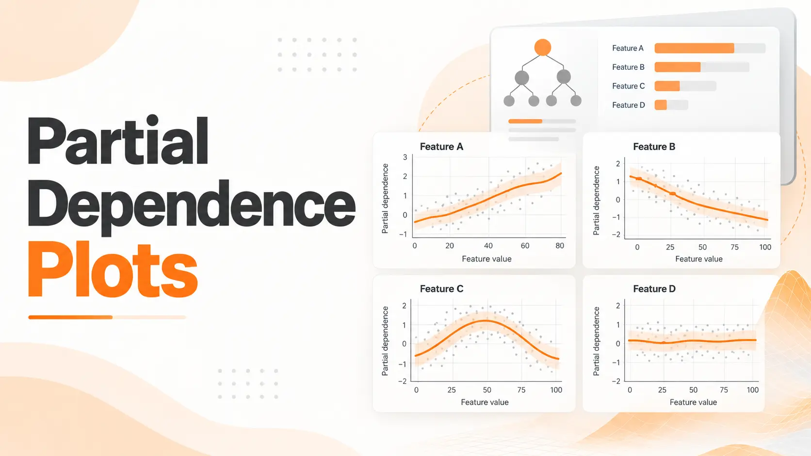
Partial Dependence Plots: Examples and Python Guide

Partial Dependence Plots (PDPs) show how a machine learning model's average prediction changes as one or two input features take different values. They help reveal whether a model has learned an increasing, decreasing, or more complex relationship between a feature and its predictions. For example, a PDP can show how predicted house prices change across different property sizes or distances from a city center.

Within Explainable AI, I find Partial Dependence Plots valuable because they provide a clear view of a model's overall behavior. However, reading the curve correctly matters more than producing an attractive chart. A PDP shows relationships learned by the model, not proof that changing a feature in the real world will cause the predicted outcome.

Partial Dependence Plot Example

Consider a machine learning model trained to predict house prices using property size, number of bedrooms, location, and distance from the city center.

Suppose we want to understand how distance from the city center influences the model's predicted property prices.

A Partial Dependence Plot can show the model's average prediction at different distances while averaging over the remaining property characteristics in a reference dataset.

Imagine the resulting plot produces these values:

5 km from the city center: $620,000

10 km from the city center: $540,000

15 km from the city center: $475,000

20 km from the city center: $460,000

These numbers are illustrative and do not come from an executed model.

The relationship is clear. As the distance increases from 5 to 15 kilometers, the model's average predicted price falls considerably. Beyond 15 kilometers, the decline becomes smaller.

I would interpret this as evidence that the model associates greater distance with lower predicted property values across the evaluated reference data.

The interesting part is not simply that the line slopes downward. It is that the slope changes.

Between 5 and 10 kilometers, the predicted price falls by $80,000. Between 15 and 20 kilometers, it falls by only $15,000.

That difference reveals how strongly the model responds across different parts of the feature range.

However, this does not mean moving a house farther from the city center would cause its value to decrease by the same amount. The plot describes the model's predictions, not a verified causal relationship.

Reading and Interpreting Partial Dependence Plots

A Partial Dependence Plot contains two main axes.

The horizontal axis represents the feature being examined. The vertical axis represents the average response of the trained model at each selected feature value.

For a house price regression model, the vertical axis can display average predicted prices.

For classification models, the vertical axis can represent predicted probabilities or decision scores, depending on the estimator and response settings.

Before interpreting any PDP, I check what the vertical axis measures. A change of 0.10 in a predicted probability has a different meaning from a change of 0.10 in a decision score.

The shape of the curve then reveals how the model responds.

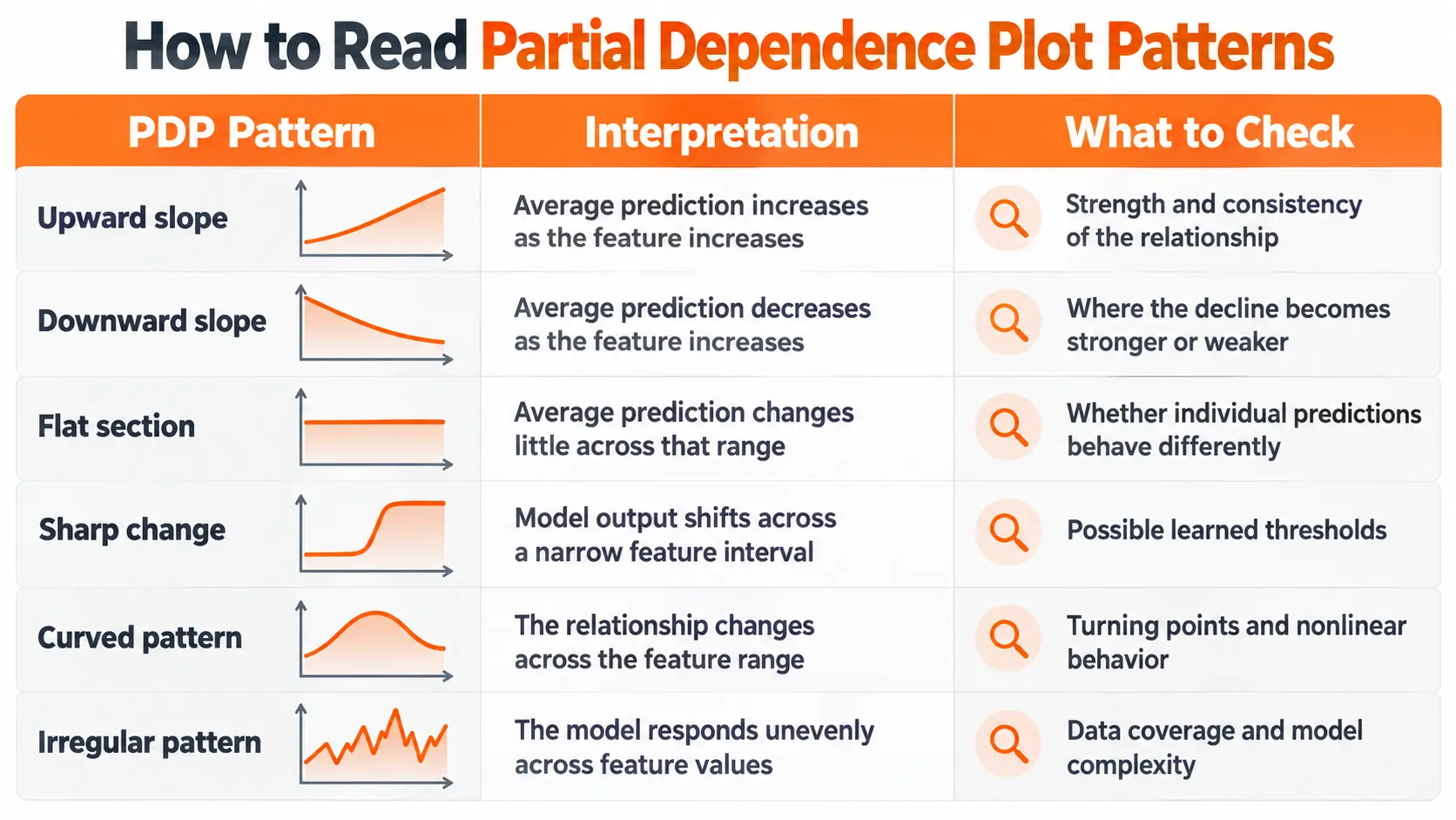
A flat PDP deserves particular attention. It does not automatically mean the feature has no influence on individual predictions.

If a feature increases predictions for one group but decreases them for another, averaging those responses can produce a nearly horizontal line.

That is why I treat the PDP as a starting point for understanding the model rather than a complete explanation of every observation.

Feature Distribution and Data Coverage

The amount of data available across the horizontal axis also affects interpretation.

Imagine a housing dataset containing thousands of properties within 20 kilometers of a city but very few properties beyond 50 kilometers.

A steep change in the PDP near 50 kilometers would deserve further investigation because the model has limited supporting observations in that region.

Feature distribution markers or a separate histogram help identify where the reference dataset contains sufficient observations.

I pay more attention to patterns in well represented regions than to isolated movements near the extremes of the feature range.

Partial Dependence Calculation

Partial Dependence Plots are calculated using predictions from an already trained machine learning model.

The process does not require retraining the model for every feature value.

Instead, the selected feature is assigned different values while the remaining features are taken from the reference dataset.

Return to the housing example.

Suppose the selected feature is distance from the city center, and the first evaluation value is 5 kilometers.

The calculation replaces the distance value in every reference observation with 5 kilometers. The remaining property characteristics stay unchanged.

The model then generates predictions for these modified observations.

Those predictions are averaged to obtain the PDP value at 5 kilometers.

The process is repeated for other distances, producing the points that form the curve.

This method reveals how the model's average response changes across the selected feature.

It also explains an important limitation. When the selected feature is strongly related to other variables, replacing its values independently can create combinations that do not resemble observations in the original dataset.

For example, changing floor area while leaving bedroom counts unchanged can produce unrealistic property combinations.

The resulting predictions still contribute to the PDP, even when the model has limited evidence about those combinations.

Creating Partial Dependence Plots in Python

Python provides a straightforward way to create PDPs through the Scikit Learn library.

For this example, I would use a house price prediction model trained with Random Forest regression.

The process involves preparing the model, selecting the features, generating the plots, and interpreting the output.

Preparing the Model and Dataset

Start with a dataset containing property characteristics such as floor area, bedroom count, building age, and distance from the city center.

The target variable is the property price.

Separate the dataset into training and evaluation sets, then train the Random Forest model using the training data.

Before examining its behavior, evaluate the model on data that was not used for fitting.

A PDP can accurately describe the behavior of a model that makes poor predictions. Model interpretation does not replace predictive evaluation.

For this reason, I establish acceptable predictive performance before treating the PDP as useful evidence about model behavior.

Generating a PDP with Scikit Learn

Scikit Learn includes Partial Dependence visualization tools within its model inspection functionality.

After training the model, select the feature you want to investigate and provide the fitted estimator together with a suitable reference dataset.

For the housing example, I would begin with distance from the city center.

The library evaluates the model across selected distance values, averages the resulting predictions, and displays the relationship.

The horizontal axis shows distance, while the vertical axis shows the model's average predicted property price.

I would then generate another PDP for floor area.

Comparing the two plots can reveal whether the model associates larger properties with higher predictions and greater distance with lower predictions.

However, their slopes should not be compared directly without considering the different feature units and output scales.

Interpreting the Python Results

Once the plot is generated, I would examine three characteristics.

First, the overall direction of the relationship. This shows whether predictions increase, decrease, or remain relatively stable as the feature changes.

Second, the shape of the curve. Turning points, sharp changes, and flat regions reveal where the model responds differently.

Third, the distribution of the reference observations. This helps distinguish patterns supported by many observations from behavior in sparsely represented regions.

For a real project, I would preserve the preprocessing pipeline used during training. The inspection process must evaluate the model using the correct feature representation.

If categorical variables were encoded or numerical features transformed, the PDP calculation must remain consistent with those transformations.

One Dimensional and Two Dimensional Partial Dependence Plots

A PDP can describe the relationship between one feature and the model's predictions or examine two features together.

The difference affects both the visualization and the conclusions that can be drawn.

One Dimensional PDP

A one dimensional PDP examines one selected feature.

For the housing model, it could show how average predicted property prices change across different distances from the city center.

The output is represented by a line, making increasing, decreasing, and nonlinear patterns easy to recognize.

I use this format when the objective is to understand the model's overall response to a single variable.

It provides a direct starting point before examining more complex relationships.

Two Dimensional PDP

A two dimensional PDP evaluates two selected features together.

For example, floor area and distance from the city center can be examined across a grid of values.

The output is displayed as a heatmap or contour plot.

One axis represents floor area, the other represents distance, and the color or contour level represents the average model prediction.

This makes it possible to investigate whether the relationship between one feature and the prediction changes across values of the other feature.

Suppose the model associates distance with a stronger price reduction for large properties than for small properties.

A two dimensional PDP can reveal this difference through the pattern of predicted values.

I would use this view when a single feature curve does not fully explain a relationship or when a meaningful interaction between two variables needs investigation.

The result still describes the fitted model rather than establishing a causal interaction in the real world.

PDP vs ICE Plots

Partial Dependence Plots and Individual Conditional Expectation (ICE) plots examine related aspects of model behavior.

The difference is how they represent predictions.

A PDP averages predictions across the reference observations to create one curve.

An ICE plot displays a separate curve for each selected observation.

Consider a pricing model trained on apartments and detached houses.

Distance from the city center might have a strong negative relationship with predicted prices for apartments but a weaker relationship for detached houses.

A single PDP averages these patterns.

The resulting curve can hide the difference between the two property categories.

ICE plots make those individual relationships visible.

When several ICE lines move in different directions, the model's response depends on characteristics of the observations being examined.

Scikit Learn can display PDP and ICE curves together, allowing the average trend to be compared with individual model responses.

I would examine ICE whenever the PDP appears unexpectedly flat or when different observations are likely to have distinct relationships.

This provides a more detailed perspective without replacing the original PDP.

PDP vs Accumulated Local Effects

Accumulated Local Effects (ALE) plots offer another method for examining the relationship between features and model predictions.

The distinction becomes particularly important when input features are strongly correlated.

A PDP evaluates predictions after assigning selected feature values across the reference dataset.

That can create combinations that rarely appear in real observations.

ALE uses local changes within feature intervals and accumulates their effects.

This reduces reliance on unrealistic combinations produced by independently varying correlated features.

Consider the relationship between floor area and bedroom count.

Larger homes tend to contain more bedrooms. A standard PDP can evaluate a very small property while retaining a bedroom count associated with much larger homes.

ALE focuses on changes within observed feature regions, reducing this particular problem.

I would investigate ALE when strong correlations make a PDP difficult to interpret reliably.

The two methods also differ in their output interpretation. A PDP displays the average model response, while a centered ALE plot displays accumulated changes relative to a reference level.

Neither method establishes causality.

Partial Dependence Plot Limitations

Partial Dependence Plots provide useful summaries, but their conclusions depend on the model, the reference data, and the relationships between features.

Correlated Features

Correlated features create one of the most important limitations.

When a selected feature is changed independently, the resulting observations can violate relationships present in the original data.

The model then generates predictions for combinations it may not have encountered during training.

Those predictions can distort the average relationship shown by the PDP.

I would inspect feature correlations before relying on the resulting curve, especially when the variables describe closely related characteristics.

Averaging Individual Differences

A PDP summarizes the average response of the model.

If different observations have opposing relationships, their contributions can cancel each other out.

This can create a flat curve even when the feature influences many individual predictions.

ICE plots help reveal those differences, while separate analyses of relevant groups can provide additional context.

A PDP should not be treated as proof that every observation responds in the same way.

Interpreting Predictions as Real World Effects

A PDP describes the trained model's prediction function, not an experiment in the real world.

For example, the housing model may associate greater distance from the city center with lower predicted prices.

That relationship can reflect other location characteristics, differences between neighborhoods, and patterns present in the training data.

Changing one feature inside the model does not reproduce the real consequences of changing that characteristic.

I would describe PDP findings as relationships learned by the model rather than causal effects.

Using PDPs to Evaluate Machine Learning Models

Partial Dependence Plots can reveal unexpected patterns that deserve closer investigation during model evaluation.

For example, suppose a house price model predicts sharply higher prices for properties with extremely small floor areas.

That result might reflect unusual training observations, interactions between features, or an unstable relationship learned by the model.

I would examine the underlying data before deciding whether the behavior represents a modeling problem.

Another useful application is comparing model versions.

Suppose a new model achieves better predictive accuracy after additional features or training data are introduced.

Generating PDPs for the original and updated models can reveal whether their learned relationships have also changed.

For a meaningful comparison, I would use the same reference dataset, selected features, and output scale.

This makes it easier to identify changes in model behavior rather than differences introduced by the evaluation setup.

PDPs are especially useful when a model needs to be reviewed by people who understand the application but do not work directly with its internal algorithms.

A readable plot can make a complicated relationship easier to discuss, provided its limitations are explained.

Conclusion

Partial Dependence Plots help reveal how a machine learning model's average predictions respond to changes in individual features or combinations of features.

They are valuable for identifying nonlinear relationships, investigating unexpected model behavior, and comparing learned patterns across model versions.

I would begin with a clearly defined feature, examine the curve and its underlying data distribution, and then check whether correlations or individual differences affect the interpretation.

When a PDP hides important variation, ICE provides a closer view of individual observations. When correlated features create unrealistic combinations, ALE offers another perspective.

The goal is not simply to produce a chart. It is to understand what the model has learned and recognize where that interpretation remains reliable.

FAQ

Can I use PDPs with XGBoost or neural networks?

Yes. PDPs can be generated for XGBoost, neural networks, and other predictive models when an appropriate prediction interface is available. The model must accept the modified observations and return consistent outputs. Computational requirements depend on the estimator and the number of evaluations.

Why does my PDP change when I use a different dataset?

A PDP depends on the reference observations used to calculate average predictions. Changing the dataset changes the distribution of feature combinations over which the model responses are averaged. Even with the same trained model, different reference datasets can produce different curves.

Can I create PDPs for categorical variables?

Yes. Categorical PDPs evaluate the model at different category values rather than across a continuous numerical range. The visualization can use discrete bars or category positions. Correct feature identification and preprocessing are essential for meaningful results.

Can I add confidence intervals to a PDP?

Uncertainty bands can be estimated through procedures such as bootstrapping reference observations or refitting models on resampled training data. These approaches measure different sources of variation and require separate interpretation. A shaded interval should not be presented as a formal confidence interval without defining how it was calculated.

Why are the feature labels on my PDP different from my original dataset?

This can happen when preprocessing changes the feature representation before the model receives the data. Encoding categorical variables, scaling numerical values, or transforming columns can alter the displayed feature names and values. The plot must be connected to the correct feature representation, and the labels should reflect the data being evaluated.