Continuous Batching for LLMs: How It Works and Improves Throughput

Continuous Batching for LLMs is an inference scheduling technique that allows new requests to join an active batch as other requests finish generating tokens. Unlike traditional batching, it does not require every request in a group to finish before processing new ones. The result is better GPU utilization and higher throughput when serving multiple requests.

The important detail is that continuous batching improves how requests share computing resources, not the underlying intelligence of the model. Its effectiveness depends on request scheduling, available GPU memory, and the balance between prompt processing and token generation.

How Continuous Batching Works in LLMs

Large language models generate responses token by token. A request first passes through the prefill stage, where the model processes its input prompt. It then enters the decode stage, generating additional tokens until the response is complete.

The challenge appears when several users submit requests with different output lengths.

One request might need 20 output tokens, while another requires 500. If both belong to a fixed batch, the shorter request finishes long before the longer one.

Continuous batching solves this scheduling problem by changing which requests participate in model execution as generation progresses.

Instead of keeping the same group together until every response is complete, the scheduler checks the active requests at each generation iteration. Completed requests leave the batch, and waiting requests become eligible for admission.

The process follows three operations:

1. Schedule active requests. The inference engine selects requests that can execute within the available token and memory budgets.

2. Execute the batch. The GPU processes the scheduled prefill or decode work for those requests.

3. Update the batch. Completed requests release their resources, allowing the scheduler to consider waiting requests for subsequent iterations.

This scheduling approach is also known as Iteration Level Scheduling or In Flight Batching.

The key distinction is that batch membership can change during generation rather than remaining fixed for the entire response.

A Practical Continuous Batching Example

Consider an inference server that can schedule four active requests under its current resource limits.

Three requests begin decoding together:

Request A: Needs 2 output tokens.

Request B: Needs 5 output tokens.

Request C: Needs 3 output tokens.

A fourth request, D, arrives while the first three are running.

During the first decode iteration, A, B, and C each generate a token.

During the second iteration, A generates its final token and leaves the active batch.

In a fixed batch, the server continues processing B and C without admitting D into that batch. D remains waiting until the existing batch completes.

With continuous batching, the scheduler can admit D after A finishes, provided that the required compute and KV cache capacity are available.

D must complete its prefill processing before joining the decode workload. A compatible scheduler can coordinate that work while B and C continue generating their responses.

When C finishes, another position becomes available. B continues generating until its fifth token completes.

This example explains the main efficiency gain: a completed request no longer forces the server to leave usable batch capacity idle while longer responses finish.

Continuous batching does not make each token inherently less expensive to calculate. It allows the system to perform more useful work with the available execution capacity.

Continuous Batching vs Static Batching

The difference between batching strategies becomes important when requests arrive at unpredictable times and produce responses of different lengths.

Static batching creates fixed groups. Dynamic batching adjusts when a group begins processing. Continuous batching goes further by updating the active workload during generation.

The following comparison shows how these approaches handle incoming requests.

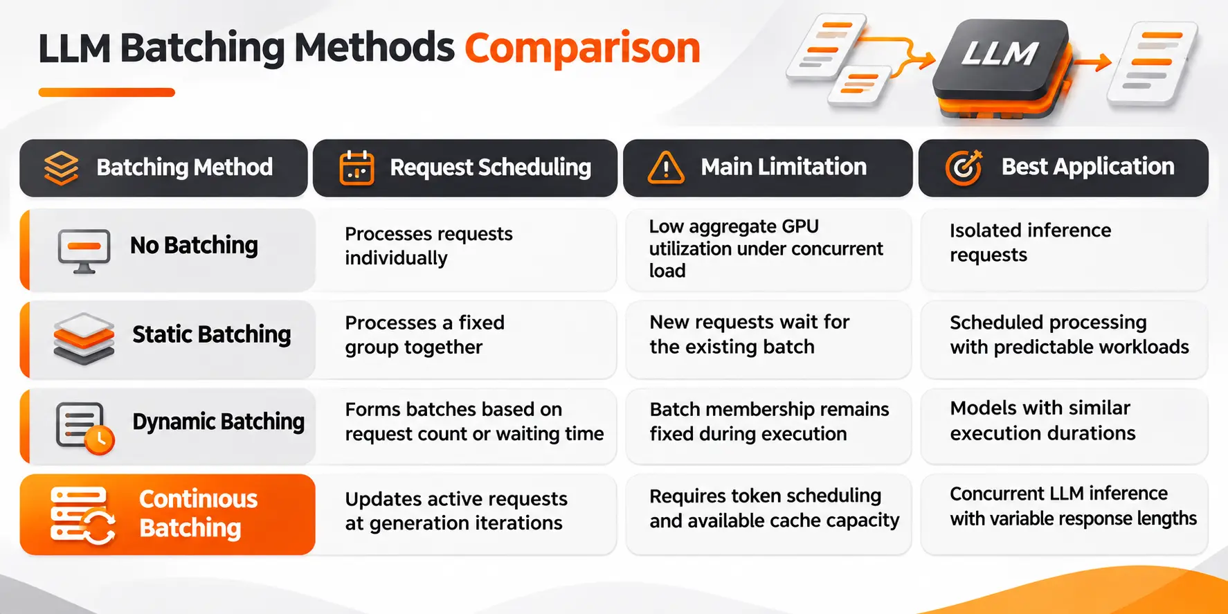
Dynamic batching deserves particular attention because the terminology differs across frameworks.

In conventional dynamic batching, a scheduler collects requests until a batch reaches a size limit or a waiting threshold. Once execution starts, the group remains fixed.

Continuous batching allows completed sequences to leave and new sequences to enter during generation.

Some technical literature uses Dynamic Batching to describe Iteration Level Scheduling. The terminology should therefore be interpreted alongside the actual scheduling behavior.

For autoregressive language models, the ability to update batches during decoding is what makes continuous batching especially valuable.

Continuous Batching Throughput and GPU Utilization

The primary performance advantage of continuous batching is higher useful throughput under concurrent workloads.

Throughput describes the amount of work a serving system completes over time. For LLM inference, it can be measured through completed requests per second or generated output tokens per second.

These measurements are related but not interchangeable.

A system generating long responses can produce many output tokens while completing fewer requests. A system handling short answers can complete more requests with a lower total output token count.

Continuous batching improves resource utilization by allowing multiple active sequences to share model execution.

During decoding, the model repeatedly accesses its weights to generate new tokens. Processing several sequences in the same execution iteration allows that work to be shared across requests.

When batch capacity is left unused, the GPU performs less useful work than it could support.

By admitting additional requests as others complete, the scheduler reduces wasted opportunities for concurrent execution.

Throughput Does Not Equal Faster Individual Responses

One distinction matters more than the headline throughput improvement.

Higher throughput does not guarantee lower latency for every request.

Adding concurrent sequences increases the amount of work performed during each execution iteration.

Although this improves aggregate efficiency, larger active batches also consume more GPU resources.

The time required to generate an individual token can increase as the workload grows.

For an interactive application, the goal is not simply to maximize tokens per second. The system must also deliver its responses within the required latency limits.

This is why we should examine throughput and latency together rather than treat either measurement as a complete performance result.

Continuous Batching Latency and Scheduling Tradeoffs

Two measurements are particularly useful for evaluating the user experience.

Time to First Token (TTFT) measures the delay before the first generated token becomes available.

Time per Output Token (TPOT) measures the average time between generated output tokens after the first.

These metrics respond to different parts of inference scheduling.

TTFT includes the effect of waiting for admission and processing the input prompt. TPOT reflects the pace of subsequent token generation.

A scheduling policy that admits large prompts aggressively can reduce their waiting time while increasing the time existing requests spend between output tokens.

A policy that strongly prioritizes active decoding requests can preserve generation speed while making newly arriving prompts wait longer.

Neither behavior is universally preferable.

For an interactive assistant, users need both a responsive first token and consistent output streaming.

For document processing, aggregate completion capacity can matter more than the time taken to display each individual token.

My preferred way to evaluate a scheduling change is to compare these two latency measurements separately. A single average response time conceals which stage actually improved.

Request Queueing and Traffic Bursts

Continuous batching also depends on how requests arrive.

At low traffic, the GPU can have enough capacity to process each request without competing with others. In that situation, continuous batching provides little opportunity to increase concurrency.

Under heavy traffic, the scheduler receives more requests than it can admit immediately.

The excess requests remain queued until computing and memory resources become available.

If incoming work consistently exceeds the server's sustainable processing capacity, the queue grows regardless of the batching strategy.

Continuous batching improves how the available capacity is used. It does not create unlimited capacity.

This distinction matters when evaluating production latency during traffic spikes.

KV Cache and Batch Capacity

Continuous batching relies on more than available computing power.

Each active autoregressive sequence retains Key and Value tensors representing previously processed tokens. The serving system must allocate memory for this cache while requests continue generating.

Longer contexts require more cache capacity in conventional full attention models.

The relationship becomes significant when many requests are active simultaneously.

A batch with eight short sequences can consume less KV cache memory than a batch containing four very long sequences.

As a result, maximum active request count does not provide a complete picture of serving capacity.

The scheduler must consider both the number of active sequences and the memory required to process their contexts.

This is where continuous batching connects with LLM Inference Optimization. Efficient request scheduling increases useful GPU work, but memory allocation determines how much concurrency the system can sustain.

Request Admission and Memory Limits

A serving engine cannot admit every waiting request simply because another request has completed.

Admission depends on the available memory and scheduling budgets.

For example, a newly arriving request with a 16,000 token prompt places different demands on the system than one containing 200 tokens.

The longer prompt requires more initial processing and additional attention cache capacity.

If the scheduler admits more sequences than the available cache can support, the engine must recover capacity through its supported memory management or request preemption mechanisms.

Preemption can interrupt an active request and require work to be recomputed or restored later.

That additional work reduces the benefit of maintaining a large active batch.

The practical lesson is to set concurrency limits according to memory consumption and request characteristics, not only the maximum number of supported sequences.

Chunked Prefill and Decode Scheduling

Continuous batching becomes more challenging when requests are in different inference stages.

Prefill processes the input prompt and performs substantial parallel computation.

Decode generates subsequent tokens, with different memory access and execution characteristics.

A long prefill operation can occupy a significant portion of an execution iteration. If active decode requests must wait for that operation, their next output tokens are delayed.

Chunked Prefill addresses this scheduling conflict.

Instead of processing an entire long prompt in one uninterrupted operation, the scheduler divides its prefill work into smaller chunks.

These chunks can be scheduled alongside decode operations, subject to the engine's capabilities and token budget.

This gives the serving system greater control over the balance between admitting new requests and maintaining the responsiveness of active ones.

Token Budget and Scheduling Priority

Consider a scheduler configured with a maximum budget of 4,096 scheduled tokens per iteration.

Assume 32 active sequences each require one decode token.

Those decode operations account for 32 scheduled token positions.

The remaining budget can be allocated to prefill work, subject to the scheduler's policy, memory availability, and execution constraints.

A long incoming prompt can be processed across multiple iterations rather than consuming an entire large prefill allocation at once.

This creates a useful scheduling tradeoff.

Giving more capacity to prefill can improve the admission and initial processing of new requests.

Allocating more scheduling opportunities to decode can improve the consistency of token delivery for active requests.

For applications with strict streaming requirements, preserving decode responsiveness deserves particular attention.

The correct token budget depends on the actual mix of prompt lengths, generated tokens, and concurrency.

Continuous Batching in Production

Production inference requires the batching strategy to work with unpredictable request arrivals, variable response lengths, and limited GPU memory.

Modern inference engines implement continuous batching through their request schedulers.

Frameworks such as vLLM, Hugging Face Transformers serving components, and NVIDIA TensorRT LLM provide capabilities for managing active sequences and dynamically scheduled work.

These implementations differ in configuration, supported models, attention kernels, and memory management.

That means two engines using continuous batching can deliver different results under identical traffic.

Configuring Request Scheduling

For a practical deployment, the most important settings concern how much work the scheduler can admit and process.

Maximum active sequences controls the number of requests that can participate in concurrent execution.

Maximum scheduled tokens limits the amount of token processing assigned to an iteration.

KV cache capacity determines the memory available for active sequence state.

Scheduling policy defines how requests are selected when available capacity is insufficient.

Chunked Prefill configuration influences the interaction between incoming prompts and ongoing decoding.

Increasing these limits without measuring the workload can create memory pressure and latency regressions.

The objective is to maintain enough concurrent work to use the GPU efficiently without allowing the active workload to exceed sustainable execution capacity.

A Practical Deployment Scenario

Consider a customer support assistant that receives a mixture of short questions and complex troubleshooting requests.

Short questions produce brief responses. Troubleshooting requests produce longer explanations.

With a fixed batch, completed short requests leave unused capacity while long responses continue generating.

Continuous batching allows the server to admit additional customer requests as earlier requests finish.

However, simply increasing concurrency does not establish that the assistant delivers better service.

If queueing increases or active requests generate tokens too slowly, users can experience longer delays despite higher aggregate throughput.

The deployment must therefore be evaluated against both processing capacity and the application's response time requirements.

Measuring Continuous Batching Performance

The most reliable evaluation compares the same model and workload under clearly defined scheduling configurations.

The comparison should preserve the model weights, numerical precision, GPU hardware, input lengths, and output generation settings.

The following measurements provide the clearest picture:

Request Throughput: The number of completed requests per second.

Output Token Throughput: The number of generated output tokens per second across the serving system.

TTFT: The delay before users receive the first generated token.

TPOT: The time required to generate subsequent tokens.

P95 and P99 Latency: The response times experienced by requests near the slow end of the latency distribution.

GPU Memory Usage: The memory required for model execution and active sequences.

Queue Waiting Time: The interval between request arrival and admission to execution.

Each metric exposes a different limitation.

A system with high token throughput but excessive queueing is not delivering a satisfactory interactive experience.

Likewise, a configuration with excellent latency for one request might fail to sustain production traffic.

Benchmarking With Realistic Concurrency

A useful benchmark needs more than a fixed collection of prompts submitted at the same moment.

Real applications receive requests over time. They also process prompts and generate responses with different lengths.

I would structure the evaluation around three traffic conditions.

First, measure performance with very low concurrency. This establishes the execution baseline without significant competition between requests.

Second, increase concurrent traffic while keeping input and output characteristics consistent. This shows how throughput and latency change as the scheduler becomes busier.

Third, introduce a realistic mixture of short prompts, long prompts, brief responses, and extended generations.

The third test is particularly important because variable sequence lengths are central to the scheduling problem continuous batching addresses.

Goodput and Operating Cost

Raw throughput is not the only useful performance result.

Goodput measures work completed while satisfying defined service requirements.

For example, a deployment can process more requests per second while allowing too many requests to exceed a latency limit.

In that situation, greater throughput does not translate into greater useful service capacity.

The relevant operating point is the configuration that completes the most acceptable work within the required latency and resource limits.

That measurement also supports cost analysis.

If a GPU instance completes more qualifying requests during the same operating period, the infrastructure cost per successful request decreases, assuming the instance cost and other relevant expenses remain unchanged.

Continuous Batching for Different LLM Workloads

Continuous batching is most valuable when several requests compete for execution and their generation lengths differ.

Interactive assistants, coding tools, and applications supporting multiple users present this scheduling pattern.

Each request advances independently, allowing the scheduler to replace completed sequences while others continue.

For a single request with no competing traffic, there is no additional request to admit into the batch. The technique therefore provides no concurrency advantage in that condition.

For large offline processing jobs, continuous batching can still improve capacity, but strict interactive latency constraints are less important. Larger scheduled workloads can be evaluated according to total completion time and hardware efficiency.

The workload should determine the configuration.

A scheduling policy designed for a high volume document processing service should not be transferred unchanged to an interactive assistant that needs immediate token streaming.

Continuous Batching and Efficient LLM Serving

Continuous batching improves LLM serving by allowing the active execution workload to change during token generation.

Instead of treating a batch as a fixed group of requests, the scheduler continuously makes room for new work as existing sequences complete.

This helps maintain GPU utilization and increase aggregate inference throughput under concurrent traffic.

The improvement is constrained by available KV cache memory, token processing budgets, scheduling policies, and competition between prefill and decode work.

For practical deployment, the decision should be based on measured throughput, queueing delay, TTFT, TPOT, and memory consumption.

Final Thoughts

Continuous batching makes LLM serving more efficient by allowing new requests to enter the execution process as others finish. Its greatest advantage appears when multiple users submit requests with different response lengths, where fixed batching leaves valuable GPU capacity unused.

However, higher throughput alone does not guarantee better performance. The real measure of success is how well the system balances request capacity, token generation speed, and memory consumption. For production workloads, continuous batching delivers its value when GPU resources are used efficiently without compromising the response times users expect.

FAQ

Can continuous batching handle requests with different temperature settings?

Yes, when the inference engine supports individual sampling configurations for requests within the same batch. Each sequence retains its own generation settings, including temperature and stopping conditions. The runtime must apply those settings independently while processing the shared execution workload.

Can I run two different LLMs in the same continuous batch?

Standard continuous batching groups execution for a shared model rather than combining unrelated model weights into one operation. Different base models require separate execution arrangements unless a specialized runtime supports another architecture. Compatible LoRA adapters can be served together in frameworks that explicitly support concurrent adapter execution.

What happens if someone cancels a request halfway through generation?

The application must communicate the cancellation to the inference server. Once the scheduler processes the cancellation and any active execution reaches a safe completion point, the request can be removed from scheduling and its allocated sequence resources released. Cancellation behavior depends on the serving implementation.

Does continuous batching work with beam search?

Support depends on the inference engine. Beam search maintains multiple candidate sequences for a request, increasing the amount of state and scheduling work involved. A runtime must explicitly support the required decoding strategy and memory management before it can execute that workload through its continuous batching scheduler.

Do I need to fine tune my LLM to enable continuous batching?

No. Continuous batching is a serving and scheduling capability rather than a modification to the model's learned parameters. It requires a compatible inference engine and appropriate runtime configuration. Model training or fine tuning is not a prerequisite for using the technique.